
MMME4008 Integrated Systems Analysis Autumn 2025 Coursework, University of Nottingham Malaysia (UNM)
Assignment Type
Individual Assignment
Subject
MMME4008 Integrated Systems Analysis
Uploaded by Malaysia Assignment Help
Date
11/08/2025
Autumn 2025 Coursework
Equality, Diversity and Inclusion (EDI) framework is an integral part to the identity and culture of the Department of Mechanical, Materials and Manufacturing Engineering at the University of Nottingham Malaysia. The Department is committed to creating an inclusive environment for all members of staff and students, regardless of their background, identity or experience.
Date of announcement: 3rd of November, 2025
Due date for submission: 9th of December, 2025 by 3 pm
Stuck in This Assignment? Deadlines Are Near?
System description
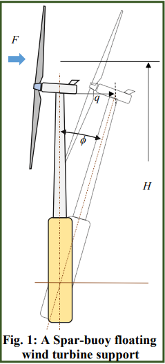
Figure 1 shows a floating wind turbine of spar-buoy type. These floating supports for wind turbines achieve stability by having a centre of mass below the centre of buoyancy (i.e. the centre of gravity of the displaced F water).
Spar-buoy floating arrangements are considered by some to be suitable for very deep water. They are relatively compliant in “pitch”. That is to say, when the wind blows and exerts a downwind thrust force on the rotor of q the wind turbine, the entire structure rocks backwards a little bit. As the structure is moving backwards relative to the oncoming wind, the relative wind speed reduces and so a coupling arises between the thrust force, F(t), f acting on the turbine and the angle of tilt, f(t), of the platform. This coursework is based on modelling the dynamics of such a floating wind turbine platform and applying the methods taught within MMME4008.
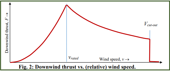
The downwind thrust on a wind turbine rotor is not a simple function of the wind speed, v(t). Every modern wind turbine has a particular fixed rated wind speed vrated. For wind speeds lower than the rated wind speed (v(t) < vrated), the turbine controller tries to extract the maximum available power from the air and this results in a downwind thrust that is proportional to the square of the wind speed, 𝐹(𝑡) = 𝑎 × 𝑣(𝑡)!. By contrast, for wind speeds higher than the rated wind speed (v(t) > vrated), the turbine is not able to absorb all of the power available and the controller must deliberately spill some power by pitching the blades suitably. This results in a different downwind force relationship … 𝐹(𝑡) = 𝑎 × 𝑣’⁄𝑣(𝑡). Figure 2 below shows a typical relationship “#$%& between wind speed and the downwind thrust force acting on a wind
Overall requirements
The requirement of this coursework is to understand this floating wind turbine as a simple dynamic system, to simulate its behaviour as wind-speed changes using SIMULINK and to analyse its behaviour at two different equilibrium states using methods taught in the course.
The submission document should be based on what is explicitly asked for in this coursework specification. The primary material being marked is the submission document – although you are asked to submit your Simulink models also. It is necessary to be able to open the Simulink models submitted using the version of MATLAB presently installed on University computers.
There are no additional marks for long submission documents, though.
Files provided to you – and what they do
| CW_Spec.pdf
|
: | This file. It contains the coursework specification. |
| f_diesel.m | : | A MATLAB function not directly related to this coursework but supplied to help illustrate |
|
|
how a SIMULINK model can call a MATLAB function. | |
| f_thrust.m | : | An MATLAB function that is not complete. You should complete this function by |
| modifying each line of code carrying the comment % Modify this line | ||
| In some cases, the modification simply involves you inserting the appropriate | ||
|
|
numerical values. In the remaining cases, you should insert the correct formula. | |
| sim_diesel.slx | : | A SIMULINK model calling the function f_diesel.m. |
| As well as showing how to call an Interpreted MATLAB Function in SIMULINK, | ||
| this also shows how to transfer data into the MATLAB workspace so that you can | ||
|
|
obtain plots using MATLAB directly. | |
| stud_data.xls | : | An EXCEL spreadsheet containing one unique row of data for each student. |
|
|
Each row contains (in this order) … {vrated, a, J, k, c, H, p, q…} | |
| start_here.m | : | A MATLAB script. This opens up a SIMULINK model of the diesel engine only, |
| (<sim_diesel.slx>) and then runs the model and plots both W and q vs. time. You might | ||
| choose to copy and then modify this so as to use it as a way to open and run your own | ||
| SIMULINK model. You can run <start_here.m> either by clicking the big green | ||
| arrowhead in the top toolbar of the editor or else by just typing >>start_here | ||
|
|
at the MATLAB command prompt). | |
Get Solved Your Assignment(variable) and Earn A+ Grade!
What to submit
Submit your coursework via MOODLE as a ZIP file. This ZIP-file should contain the coursework submission document itself (in portable document format, otherwise known as pdf). All files that you used in the coursework are also needed. Name it as submission.pdf.
Important Please make clear on the first page of the submission document which student you are by identifying which row of the spreadsheet applies to you. For the purposes of your submission document, please refer to this number as the “SID_No”. (Student Identification number). It is important to use the parameter values specified in the row number assigned to you; this would be checked during the marking process.
The coursework submission document should comprise:
a) A response to Task 1 (up to half a page)
b) A response to Task 2 (the corrected function, <f_thrust.m>, and three numerical answers) Ø
c) A response to Task 3 (up to half a page). This should include an explanation of how you applied an algebraic or iterative approach to finding the two equilibrium conditions and a description of the equilibrium condition comprising {𝐹(.*, 𝜙(.*, 𝑞(.*}. Ø
d) A response to Task 4 which should comprise
-
- a legible view of the Simulink model (on a single page)
- an explanation in text of how you have applied the initial conditions, briefly, in a few sentences – the plot of q(t) vs. t.
- e) A response to Task 5 (1 page) comprising
- the Simulink model and – a plot of q(t) vs. t.
- f) A response to Task 6 (<2 pages) containing
- an explanation of how you determined the state-space representation for one condition (you need not repeat this explanation) and
- how you used the state-space representation to determine how q(t) varies with respect to time, t. – how the eigenvalues of the A matrix for the equilibrium condition at v(t) @ 14 was calculated and their interpretation.
- the graph of q(t) vs. t from the new SIMULINK model and a commentary on any connection between the eigenvalues and this graph.
These responses would correspond to the bullet points, starting with a ‘ ’ symbol, shown in boxes throughout this submission document.
Equations defining the system
The following equations define the behaviour of this system. In these equations, a dot above a quantity indicates differentiation with respect to time. The angle 𝜙 is measured in radians.
1) Define: 𝑤(𝑡) ≔ 𝑣(𝑡) − 𝐻 × 𝑐𝑜𝑠(𝜙) × 𝜙̇(𝑡)
2) If 𝑤!“#$”#, 𝐹(𝑡) = (𝑎 × 𝑣%&#’()!“#$”#)7
Otherwise if 𝑤 𝑣%&#’(, 𝐹(𝑡) = 𝑎 × 𝑣%&#’()⁄𝑤(𝑡)
Otherwise 𝑤 𝑣%&#’( and 𝐹(𝑡) = 𝑎 × 𝑤(𝑡)* × 𝑠𝑖𝑔𝑛(𝑤(𝑡))
3) 𝐽 × 𝜙̈(𝑡) + 𝑐 × 𝜙̇(𝑡) + 𝑘 × 𝜙(𝑡) = 𝐹(𝑡) × 𝐻 × 𝑐𝑜𝑠2(𝜙)
4) 𝑞 = 𝐻 × 𝑠𝑖𝑛(𝜙)
THE COURSEWORK REQUIREMENT – 6 TASKS
Task 1.
l Identify and state what the state variable, rate variable and input is.
[10 marks]
Task 2.
| l | Correct the necessary lines of code present in the supplied function, <f_thrust.m> and present that function in your submission document. Then call that function directly from the MATLAB for three different wind speeds: {3m/s, 9.5m/s, 28m/s}. |
| l | Report the results.
HINT: To get the answer for 9.5m/s, type … f_thrust( 9.5) at the MATLAB command prompt. |
[10 marks]
Task 3.
| l | Without using SIMULINK, determine an equilibrium condition for the dynamic system at the wind speeds 9.5m/s and 14m/s. |
| l |
Report the following steady values, 𝐹(.* = 𝜙(.* = 𝑞(.* = |
HINT: There is no “closed-form” solution here so you will have to apply an iterative approach of some sort. A manual iteration process is fine. You do not have to write any code to implement an iterative solution automatically or to use any built-in iterative methods within MATLAB.
[15 marks]
Task 4
Now create a Simulink model of the system and run this model over a period of 500s with a constant wind-speed of 9.5m/s taking the initial conditions to be f(0) = 0.15 rad and 𝜙̇(0) = 0.
| l | Present the Simulink model in your submission document. |
| l | Plot q(t) vs. t . |
| l | State, in your submission document, how the initial conditions are set in the Simulink model. |
[25 marks]
Task 5
Modify the Simulink model from Task 4 so that the wind speed is now varying sinusoidally according to 𝑣(𝑡) = 9.5 + 0.2𝑐𝑜𝑠(0.2𝑡). Change the initial conditions so that f(0) = f9.5 determined from Task 3.
| l | As in the previous task, present this Simulink model in your submission document. |
| l | Plot q(t) vs. t over 500s. |
[10 marks]
Task 6
For the equilibrium condition of v(t) @ 14 m/s, by considering a truncated Taylor series expansion, analytically linearise the system about this speed, such that it is expressed in the state-space form, where v(t) is the only input, and q(t) is the only output.
| l | Report the four matrices in the state-space form. |
| l | Predict the system’s steady state response from this state-space form |
| l | Comment on system stability by calculating the eigenvalues of the A matrix and plotting q(t) versus t over 500 s for an initial condition of f(0) = (f14 + 0.001). |
[30 marks]
Get 30% Discount on This Assignment Answer Today!
Get Help By Expert
Facing trouble building your Simulink model or analysing eigenvalues for your MMME4008 Integrated Systems Analysis coursework at UNM? Don’t worry — our engineering assignment experts in Malaysia can help you finish it on time with AI-free, human-written solutions that match university rubrics. Get step-by-step help for MMME4008 Integrated Systems Analysis coursework today from the team at Malaysia Assignment Help for guaranteed high-quality results.

Recommended Assignments for You
Related University Assignments
- PSGA1011 Psychology of Human Cognition Assignment Essay 2026 | UNM
- BUSI1107 Introduction to Economics Individual Assignment 2025-2026
- PSGA1012 Personality and Intelligence Assignment | University of Nottingham Malaysia
- PSGA1009 Psychology of Individual Differences Assessment Reflective Report | University of Nottingham Malaysia
- BUSI3162 Advanced Management Accounting Individual Coursework Brief 2025-2026 | University of Nottingham Malaysia (UNM)
- MMME4008 Integrated Systems Analysis Autumn 2025 Coursework, University of Nottingham Malaysia (UNM)
- BUSI2085 Accounting Information Systems Assignment Coursework 2025-2026
- Leadership Assignment Report: Dynamic Leader Case Study on Born vs. Made Leaders and Gender Leadership Insights
- International Business Strategy Assignment: Cross-Border Issues & Strategic Solutions for a Global MNC
- Master Budgeting and Financial Analysis Assignment: Kelantan Expansion & Bursa Malaysia Investment Case Study

Convincing Features